Zillow Engineering: Behind Zillow 3D Home App and Tour - Backend Algorithms7314
Pages:
1
 WGAN Forum WGAN ForumFounder & WGAN-TV Podcast Host Atlanta, Georgia |
DanSmigrod private msg quote post Address this user | |
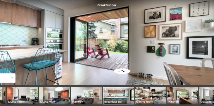 Hi All, In the article below - reprinted with the permission of Zillow - Zillow Engineering explains the recipes it uses to create Zillow 3D Homes, both for panorama generation and inter-panorama connections. While Zillow is still beta testing its 3D Home app -- used to create the Zillow 3D Home Virtual Tours for Zillow Real Estate Listings -- I could imagine that it will be rolled out across the U.S. by the end of this year (2018). Your thoughts? Best, Dan P.S. We Get Around Network Forum discussions tagged: Zillow | Zillow 3D Home --- Zillow announced 3D Home in October 2017. It allows people to view a home via 360-degree panoramas and help them grasp the “flow of the house” by clicking arrows in the panorama viewer to move from location to location. Our goal with 3D Home is to democratize the technology, allowing anyone with an iPhone to create such content without additional hardware. It’s free to use our Zillow 3D Home App, free to generate the final presentation, free to list and view it on Zillow Group home detail pages, and free to embed it on third-party broker/photographer websites. What this means for the backend algorithms is that we need to support (1) high-quality hand-held 360-degree panorama stitching, and (2) automatic and smooth inter-panorama transitions. In this article, I will explain how we tackle both problems. Capture Process Once the Zillow 3D Home app is downloaded onto the iPhone, a user can start a capture. The phone is held in front of the user to gather both the videos and the Inertial Measurement Unit (IMU) motion data. A capture starts with a panorama capture, a 360-degree spin at a user-picked location. It is followed by a link capture, where the user picks a second location and walks there. Panorama captures and link captures alternate, ending with a panorama capture to complete a floor. The process is illustrated in the top-down view in Figure 1. For a more detailed explanation of the capturing process, please refer to the official instructional guide. 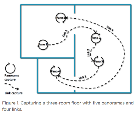 Panorama Generation Our input for panorama generation is an upright rotating video at a user-selected capturing location. We first decompose the captured video into a sequence of image frames, then stitch them spatially and blend them photometrically into a panorama, as shown in Figure 2. 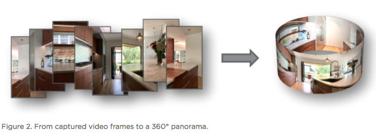 To explain the stitching process, we need to understand how two images are stitched together. As illustrated in Figure 3, we need to compute a mapping H (a 3x3 homography transformation matrix) to transform any pixel located at coordinate (x,y) in Image 2 to a new pixel location (x’, y’) in Image 1, per Equation 1.  Generally, H can be computed from at least four corresponding pixel pairs between the two images (the green arrows in Figure 3). Such pixels are called point features (the red dots in Figure 3), which are special pixels that can be uniquely identified across images. 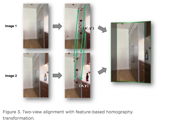 To stitch a series of images, one just needs to stitch them sequentially as described above. Easy? Not quite. Lack of Texture For real estate captures, there are many regions such as empty walls where it is difficult to find enough corresponding feature pairs (textureless regions in Computer Vision terms) needed to compute a homography. How do we robustly align such images in this case? The solution we chose is to utilize the phone’s motion data. Specifically, we obtain the relative 3D rotation R (3x3 rotation matrix) from the IMU between the camera poses of consecutive frames. Given R and the camera intrinsic matrix K following the pinhole camera model, the transformation homography matrix H can be directly computed following Equation 2, without the required feature matches.  Despite IMU data noise and other factors — such as minor translation during the image frame capturing, as shown in Figure 4 (a) — such alignment already gives us a good starting point in the general indoor environment. To compensate for the IMU rotational noise and minor translation, we then apply iterative optimization over R and K to search for better homographies such that it minimizes edge alignment error between the image pair, as shown in Figure 4 (b). Note that the shelf, sofa, and ceiling are better aligned. The Parallax Effect The parallax effect causes nearby objects to appear differently when the camera moves slightly. This effect is the basis for our human stereo vision, but it can cause problems for panorama generation. For example, objects might be occluded or appear to be in a different position in one view but not the other. Resolving the different views can cause stitching artifacts such as double/blurry edges, as seen on the lampshade in Figure 4 (b). Parallax tends to be more noticeable to objects closer to the camera location than those farther away. This is also why it normally is not an issue for outdoor hand-held panorama capturing, because outdoor scenes are normally far enough away from the phone that any parallax introduced by hand-held jitter is not noticeable. In the case of our indoor real estate applications, such hand motion cannot be ignored. To fix the parallax effect, we apply optical flow alignment that creates a nonlinear, local pixel-to-pixel warping, so that objects both close to the viewing location and at a distance are aligned in the final panorama. 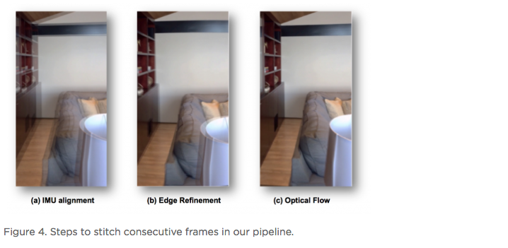 The Loop Closure The iPhone’s internal panorama mode only produces up to 240-degree panoramas. To generate full 360-degree panoramas, we need to wrap the panorama image around the end to the beginning as well, using a process called loop closure optimization. Due to hand-held capturing, we inevitably accumulate local translations between the first and last frame. So, we cannot directly use the IMU-based homography solution to align this special frame pair. Instead, we apply either feature-based homography computation as discussed in Figure 3 or an appearance-based matching (histogram matching) to improve them. Once the loop closure frame pair is decided and its transformation computed, we perform a global optimization to redistribute the local alignment errors (including loop closure) across all the panorama images. This optimization is called bundle adjustment. The effect before and after the bundle adjustment is shown in Figure 5. 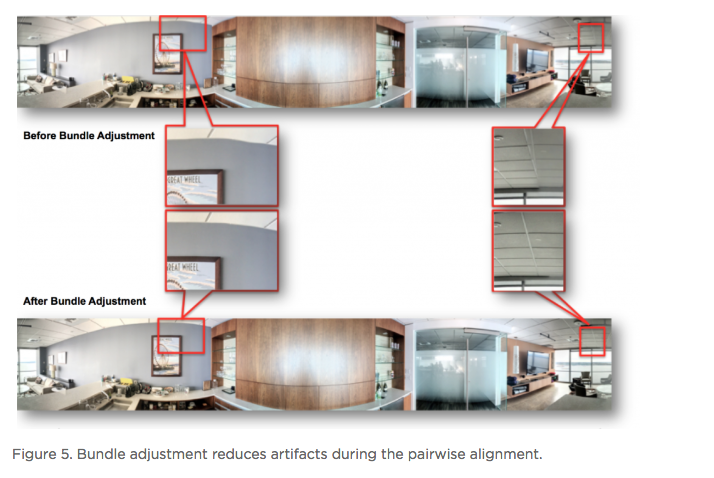 Blending and Image Enhancement So far we have aligned the panorama frames geometrically. We need to boost the image quality photometrically as well. We use a multiscale image blending approach to remove the edges introduced by a smartphone’s auto-exposure, as shown in the first rows of Figure 6. We apply a non-local exposure correction as our final enhancement to adjust underexposed regions and improve the overall brightness of the scene, as shown in the last row of Figure 6. 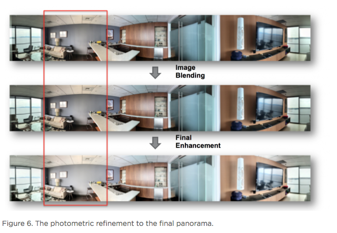 Panorama Connections Panorama connections (the annotated arrows in the topmost figure) link panoramas spatially in the 3D Home. They are immersive, clickable “portals” to other panoramas. They are also indicators of the house layout, indicating how other panoramas are located with respect to the current one. What does it mean to compute a connection? Essentially, it is to figure out the next panorama’s camera location from the current panorama. Let’s look at an example shown in Figure 7. Once we figure out Panorama 2’s camera location in Panorama 1, we can compute the departure angle of Panorama 1 to Panorama 2 (the red line in the second row). The yellow lines indicated the landing direction in Panorama 1 after jumping from Panorama 2. We call these arrival angles. Note that the departure and arriving angles exist in pairs, and they are exactly 180 degrees apart. It allows all connections in our viewers to be bi-directional and allows back-and-forth traveling between a pair of panoramas. Given Panorama 1’s camera location in Panorama 2, we can compute the departure and arrival angles in Panorama 2 as well (third row). Based on how the panorama locations are be computed, we can compute panorama connections in two ways. First, for a pair of panoramas that visually contain common regions of the scene, their locations can be computed using the Computer Vision Two-View Geometry. We call this a Pano-Visual Connection (PVC). Second, for a pair of panoramas between a link capture, their locations can be computed from the link capture’s IMU data. We call this a Pano-Link-Pano Connection (PLC). 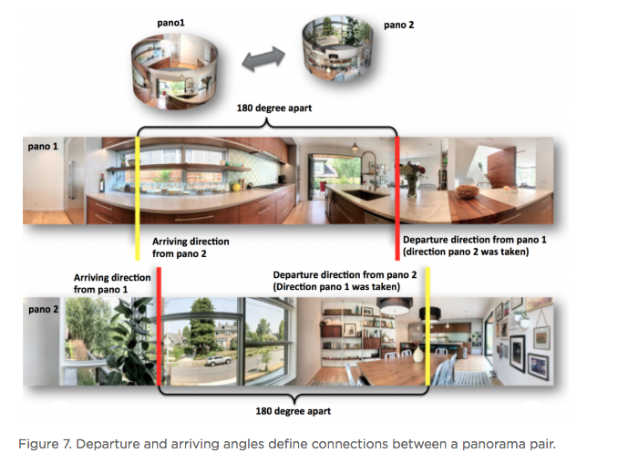 Figure 8 illustrates the relationship and differences between the captured links and the final connections presented in the 3D Home Viewer. Three PVCs are computed: panorama pairs 1 & 5 and 2 & 3 are in the same room; 2 & 5 can see each other through the door that connects the two rooms. Four PLCs are computed from the four captured links. 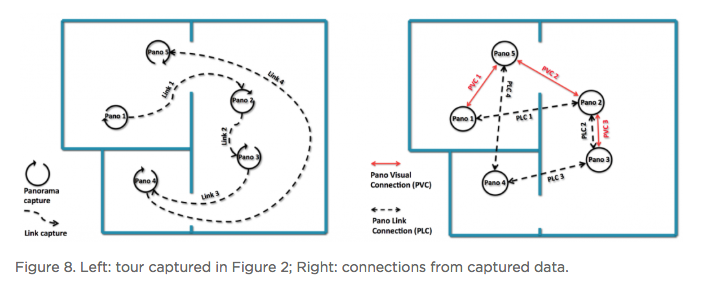 Pano-Visual Connection (PVC) computation PVCs are computed when a pair of panoramas visually contain overlapping regions. To recover the relative camera positions, we resort to the Two-View Geometry theory in Computer Vision. Simply put, this is done similarly to the frame-to-frame matching case that we described earlier in Figure 3; i.e., feature detection and cross-frame matching followed by equations solving. The differences are (1) the features are extracted and matched from the spherical panoramas; (2) the relative motion between the images is computed thanks to an estimation of a relative pose estimation using a spherical camera model parametrization; (3) the departure/arrival directions computed; and (4) the essential matrix models out-of-plane feature correspondences, as opposed to the homography matrix that only models in-plane feature transformation. The complete process is illustrated in Figure 9. Note the departure/arrival directions in Figure 9 (c) correspond to the vertical lines of the same color in Figure 7. 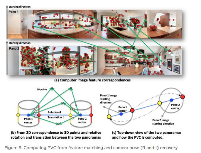 The relative pose is computed by the estimation and the decomposition of the essential matrix E into a relative rotation R and a translation t between the two cameras (Equation 3). This essential matrix E encodes a point to line mapping between two cameras (in this case, spherical cameras). R defines how the two panoramas are oriented in the world coordinate system, indicated by the gray arrows in Figure 9(c). The arrows also correspond to the left edge of the panoramas in Figure 9(a). t defines how the two panoramas are located, indicated by the panorama centers in Figure 9(c). This relative pose allows us to compute the jumping direction from one sphere to another and can bypass the link trajectory computation as described in PLC.  Pano-Link-Pano Connection (PLC) Computation PLCs are computed when a pair of panoramas are associated by a link capture. Given the accelerometer and gyroscope readings from the link capture’s IMU data, we can obtain the 3D linear acceleration and rotational speed at any arbitrary time during the link capture. From the basic physics, we know that by double integrating the linear acceleration we can get the position of the phone and the walking trajectory from one panorama to the next, as shown in Figure 10. 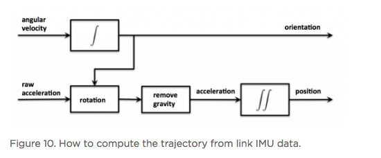 Raw IMU data has a lot of noise. If we use the signals directly, the trajectory after the double integration would quickly drift away and make the result useless. We have implemented two approaches to deal with the position drift. For the first approach, we pose the task as an optimization problem with certain constraints to minimize the impact of the system noise — starting and ending walking velocities and accelerations are zero, integrated velocities and rotations should not have sudden changes, etc. For the second approach, we train a machine-learning model to classify the walking pattern for each link capture. The model should recognize walking steps from the raw, noisy IMU accelerometer data. Similar to Figure 9 (c), Figure 11 shows the top-down view of a panorama pair connected by a link trajectory. The locations, t, of the two panoramas defined by the IMU trajectory computation mentioned previously are shown as the dark dashed curve in Figure 11. The orientation, R, computation combines three orientations: R_trajectory, the walking direction defined by the walking trajectory; R1, the direction the user walked out of in Panorama 1 with respect to the starting direction; and R2, the direction the user walked into in Panorama 2 with respect to the starting direction. R1 and R2 are visualized as the green arrows in Figure 11. 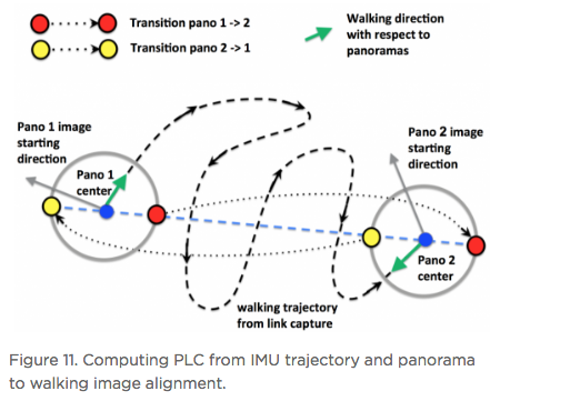 R_trajectory can be easily derived from the trajectory — the dashed blue line in Figure 11. To compute R1 and R2, we need to align the starting frame of the link video with Panorama 1 and the ending frame of the link video with Panorama 2. The idea is similar to the loop closure step in panorama generation, where we find the best alignment between the link frame with the panorama, as Figure 12 illustrates: we try to find the orientation of the Link 1 video frames with respect to Panorama 1. We try to make the computation more robust by computing a rotation (the green arrows) from multiple consecutive frames and get the consensus of rotations (the red peak) as the final rotation R1 or R2. Finally, we stack the three rotations to figure out the PLC rotation R, as in Equation 4. 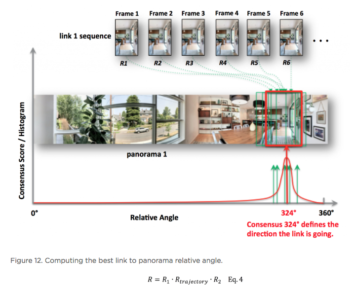 Global Optimization and Refinement We use a global optimization scheme to refine all panorama locations, panorama orientations, and link trajectories all at once so that we can create consistent angles if both PVCs and PLCs exist for any panorama pairs (e.g., Panorama 2 and 3 on the right side of Figure 8). To improve the viewing experience, we also filter out certain connections to avoid crowding panoramas with arrows. In addition, we also compute the warping factors (scaling and rotation) between a panorama pair so that after the arrow is clicked, the user will experience a smooth and accurate transition from one panorama to the next. Summary In this article, we explained the recipes we use to create Zillow 3D Homes, both for panorama generation and inter-panorama connections. In our next blog, we will share some tips and tricks to make high-quality 3D Home tours. Stay tuned! Source: Zillow Engineering (reprinted with permission of Zillow) |
||
| Post 1 • IP flag post | ||
Pages:
1This topic is archived. Start new topic?

